SHAP Analysis for NIRS Models
Overview
The SHAP (SHapley Additive exPlanations) module provides explainability for NIRS models by identifying which spectral regions are most important for predictions.
Key Design Decisions
✅ ALL Visualizations Use Binned Features
Every SHAP visualization in this module uses binned wavelengths/features, not individual points:
Spectral importance: Shows binned regions on the spectrum + bar chart
Beeswarm plot: Bins features before plotting
Waterfall plot: Bins features before showing contributions
Summary plot: Uses raw features (standard SHAP, useful for non-spectral data)
Why Binning?
Individual wavelengths are prone to:
Noise and artifacts from instrument variability
Overfitting to training set peculiarities
Misleading peaks at single points
Binning creates robust spectral regions:
Aggregates SHAP values over multiple wavelengths
Smooths out noise while preserving trends
Provides interpretable regions (e.g., “1600-1620 nm”)
Scientifically meaningful (absorption bands span ranges)
Binning Configuration
Control binning with these parameters:
shap_params = {
    'bin_size': 20,           # Wavelengths per bin (default: 20)
    'bin_stride': 10,         # Step between bins (default: 10 = 50% overlap)
    'bin_aggregation': 'sum'  # How to combine SHAP values in a bin
}
Per-Visualization Configuration
You can now specify different binning for each visualization using dictionaries:
shap_params = {
    'bin_size': {
        'spectral': 20,      # Fine detail for overview
        'waterfall': 50,     # Coarser for clarity
        'beeswarm': 30       # Medium detail
    },
    'bin_stride': {
        'spectral': 10,      # 50% overlap
        'waterfall': 25,     # 50% overlap
        'beeswarm': 15       # 50% overlap
    },
    'bin_aggregation': {
        'spectral': 'sum',      # Total importance
        'waterfall': 'mean',    # Average per wavelength
        'beeswarm': 'sum_abs'   # Absolute sum
    }
}
Aggregation methods:
'sum'- Sum of SHAP values (emphasizes cumulative effect)'sum_abs'- Sum of absolute values (ignores direction)'mean'- Average SHAP value (normalized by bin size)'mean_abs'- Average absolute value
Examples:
bin_size=20, bin_stride=10→ 50% overlap between binsbin_size=30, bin_stride=30→ No overlap (independent bins)bin_size=50, bin_stride=25→ 50% overlap with wider regions
Visualizations
1. Spectral Importance ⭐ Main Visualization
Shows which spectral regions matter most for predictions.
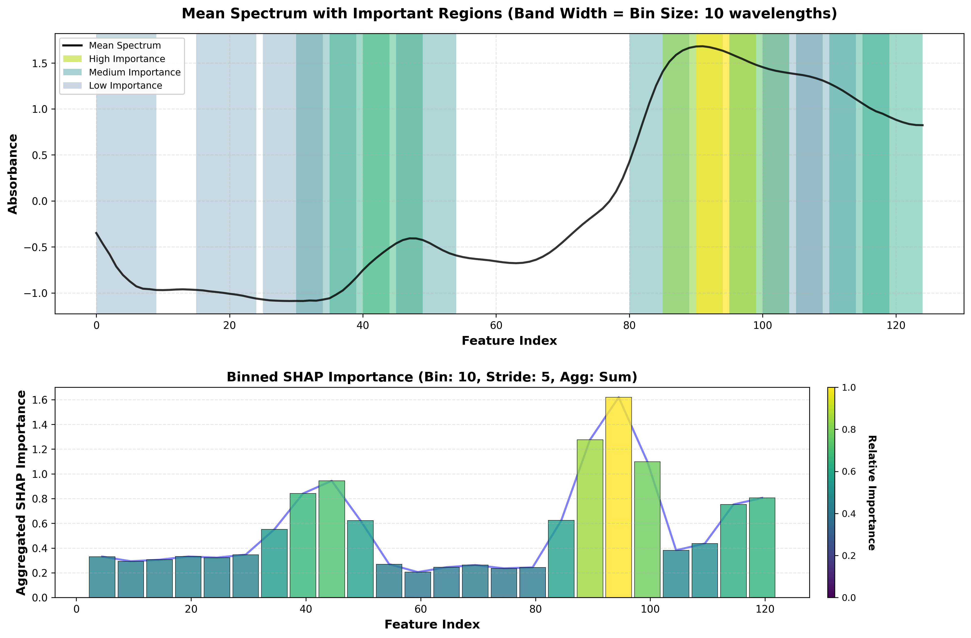
SHAP spectral importance plot showing important wavelength regions.
Top Panel - Spectrum with Regions:
Black line: Mean spectrum of your data
Colored bands (Viridis): Important regions highlighted
Light yellow/green = moderately important
Dark blue/purple = highly important
No highlight = low importance
Bottom Panel - Bar Chart:
X-axis: Wavelength (nm)
Y-axis: Aggregated SHAP importance per bin
Viridis colormap: Bars colored by importance
Blue line: Trend across spectrum
How it works:
Computes SHAP values for each wavelength
Sorts wavelengths to ensure proper ordering
Creates overlapping bins (default: 20 wavelengths, 50% overlap)
Aggregates SHAP values within each bin
Visualizes binned importance
2. Beeswarm Plot (Binned)
SHAP beeswarm showing feature value vs. SHAP impact, with binned features.
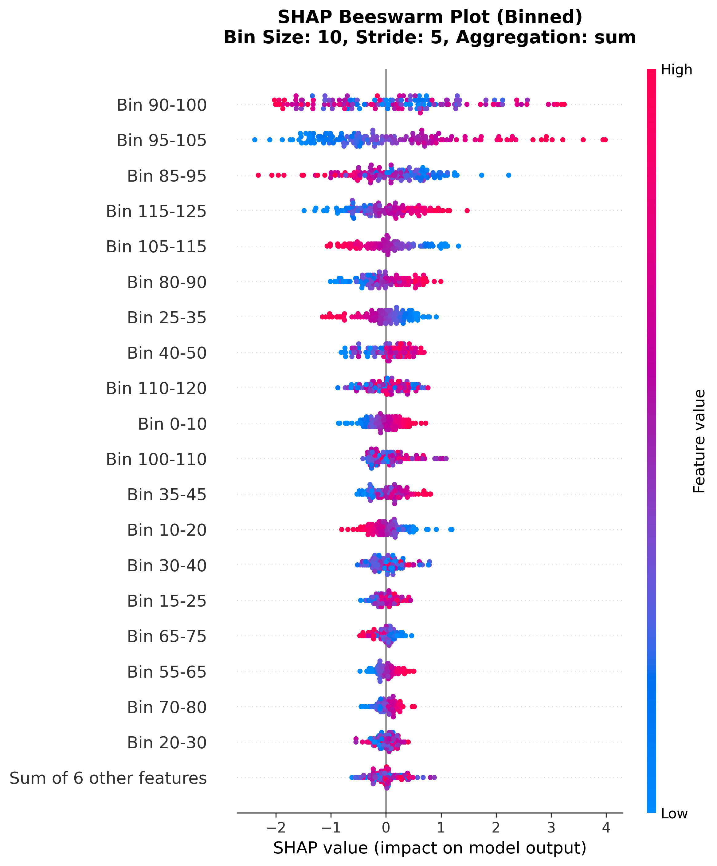
SHAP beeswarm plot showing distribution of SHAP values for binned features.
Each dot = one sample
X-axis: SHAP value (impact on prediction)
Color: Feature value (red=high, blue=low)
Y-axis: Binned wavelength regions (sorted by importance)
Interpretation:
Dense clusters = consistent behavior across samples
Wide spread = variable impact depending on sample
Color patterns = how feature values relate to SHAP impact
3. Waterfall Plot (Binned)
Shows how binned features contribute to a single prediction.
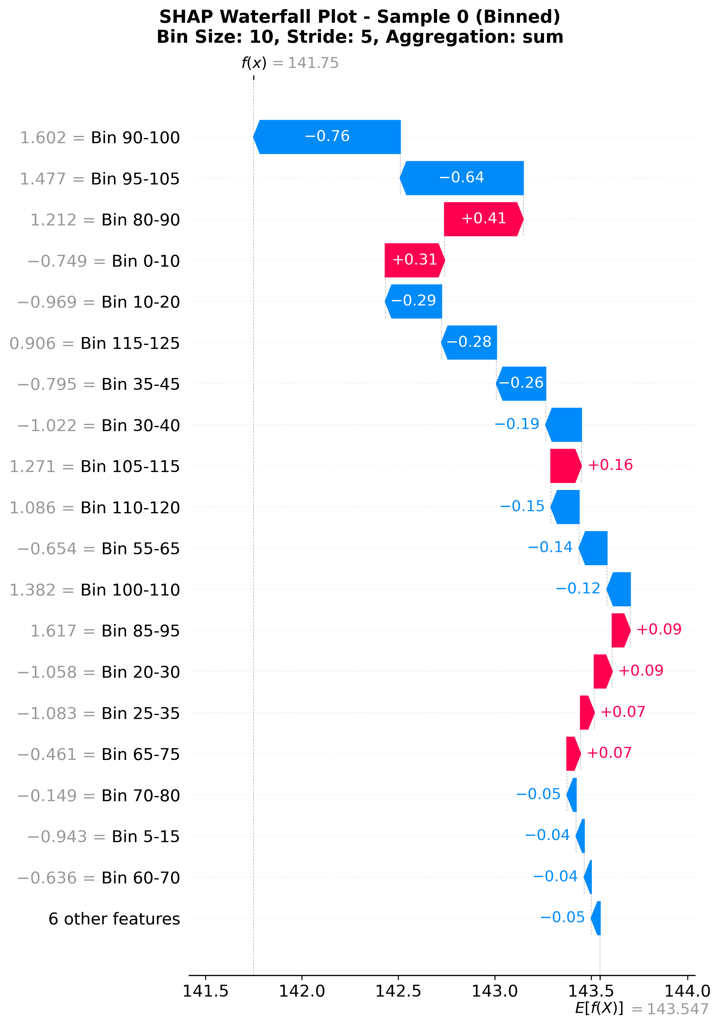
SHAP waterfall plot showing feature contributions to a single prediction.
Starts from base value (expected value)
Each bar = contribution from one binned region
Red bars = push prediction higher
Blue bars = push prediction lower
Ends at final prediction
Use for:
Understanding individual predictions
Debugging specific samples
Explaining predictions to stakeholders
4. Summary Plot (Raw Features)
Standard SHAP summary plot showing overall feature importance.
Note: This uses individual features, not binned. Useful for:
Comparing different feature types (e.g., spectra + metadata)
Standard SHAP workflow compatibility
Non-spectral data analysis
Usage
Basic Example
from nirs4all.pipeline import PipelineRunner

# Train model
runner = PipelineRunner(save_artifacts=True)
predictions, _ = runner.run(pipeline_config, dataset_config)
best = predictions.top(n=1, rank_metric='rmse')[0]

# Explain with SHAP (default binning)
explainer = PipelineRunner()
shap_params = {
    'n_samples': 200,
    'visualizations': ['spectral', 'beeswarm', 'waterfall']
}

results, output_dir = explainer.explain(best, dataset_config, shap_params)
Custom Binning (Same for All)
shap_params = {
    'n_samples': 200,
    'visualizations': ['spectral', 'beeswarm', 'waterfall'],
    'bin_size': 50,              # Wider bins
    'bin_stride': 25,            # 50% overlap
    'bin_aggregation': 'mean_abs'  # Average absolute SHAP values
}

results, output_dir = explainer.explain(best, dataset_config, shap_params)
Custom Binning (Per-Visualization)
shap_params = {
    'n_samples': 200,
    'visualizations': ['spectral', 'waterfall', 'beeswarm'],

    # Different binning for each visualization
    'bin_size': {
        'spectral': 20,      # Fine-grained spectral overview
        'waterfall': 50,     # Coarser - fewer bars for clarity
        'beeswarm': 30       # Medium detail
    },
    'bin_stride': {
        'spectral': 10,      # 50% overlap
        'waterfall': 25,     # 50% overlap
        'beeswarm': 15       # 50% overlap
    },
    'bin_aggregation': {
        'spectral': 'sum',      # Total importance per region
        'waterfall': 'mean',    # Average per wavelength
        'beeswarm': 'sum_abs'   # Absolute importance
    }
}

results, output_dir = explainer.explain(best, dataset_config, shap_params)
Why use different binning per visualization?
Spectral: Fine detail to see all important regions
Waterfall: Coarser bins → fewer bars → easier to interpret
Beeswarm: Medium bins → balance between detail and readability
All Parameters
shap_params = {
    # SHAP computation
    'n_samples': 200,              # Background samples (default: 200)
    'explainer_type': 'auto',      # 'auto', 'tree', 'linear', 'deep', 'kernel'

    # Visualizations (all support binning)
    'visualizations': ['spectral', 'summary', 'waterfall', 'beeswarm'],

    # Binning configuration - can be int/str OR dict
    'bin_size': 20,                # int: same for all, dict: per-viz
    'bin_stride': 10,              # int: same for all, dict: per-viz
    'bin_aggregation': 'sum'       # str: same for all, dict: per-viz
}
Interpreting Results
Spectral Importance
Example: Protein Prediction Model
If you see high importance in:
1600-1700 nm (dark purple band): Amide I band → C=O stretch
2100-2200 nm (dark purple band): Amide II band → N-H bend
2300-2400 nm (medium blue band): C-H combinations
✅ Model learned chemically meaningful features!
Troubleshooting:
High importance in unexpected regions → May indicate artifacts or preprocessing issues
Uniform importance everywhere → Model might be overfitting or data is too noisy
Importance at spectrum edges → Check for edge effects from preprocessing
Beeswarm/Waterfall (Binned)
Look for:
Consistent patterns → Reliable spectral regions
Variable contributions → Context-dependent regions
Strong push in one direction → Dominant spectral features
Scientific Interpretation
Validation Strategy
Run SHAP analysis on best model
Identify top regions from spectral importance
Cross-reference with chemistry:
Do important regions match known absorption bands?
Are they consistent with the target property?
Compare models: Do different models rely on similar regions?
Example Workflow
# Explain top 3 models
top_models = predictions.top(n=3, rank_metric='rmse', rank_partition='test')

for model in top_models:
    results, output_dir = explainer.explain(model, dataset_config, shap_params)
    # Compare which regions are consistently important
Advanced Usage
Experiment with Bin Sizes
# Try different bin sizes to find optimal resolution
for bin_size in [10, 20, 30, 50]:
    shap_params['bin_size'] = bin_size
    shap_params['bin_stride'] = bin_size // 2  # Always 50% overlap

    results, _ = explainer.explain(best, dataset_config, shap_params)
    # Compare results
Compare Aggregation Methods
for agg in ['sum', 'sum_abs', 'mean', 'mean_abs']:
    shap_params['bin_aggregation'] = agg
    results, _ = explainer.explain(best, dataset_config, shap_params)
    # See which gives clearest insights
Technical Details
SHAP Value Calculation
Select appropriate explainer (Tree/Linear/Deep/Kernel)
Compute SHAP values for each sample × feature
Store raw values for later binning
Binning Process (for spectral/beeswarm/waterfall)
Extract wavelengths from feature names (λXXX.X format)
Sort features by wavelength
Create overlapping bins:
bin_start = 0, bin_stride, 2*bin_stride, ...
bin_end = bin_start + bin_size
Aggregate SHAP values per bin using selected method
Create bin labels (e.g., “1650.0-1670.0 nm”)
Generate visualization with binned data
Explainer Selection
Tree models (RF, GBM, XGBoost): TreeExplainer (fast, exact)
Linear models (Ridge, Lasso, PLS): LinearExplainer (fast)
Neural networks: DeepExplainer
Others: KernelExplainer (slower but universal)
Plotting Behavior
All plots are blocking - execution pauses until you close the plot window. This allows you to:
Examine each visualization carefully
Save screenshots manually
Compare visualizations side-by-side
Plots are also automatically saved to:
results/<dataset>/<config>/explanations/<model_id>/
  ├── spectral_importance.png
  ├── summary.png
  ├── waterfall_binned.png
  └── beeswarm_binned.png
FAQ
Q: Why aren’t individual wavelengths shown in beeswarm/waterfall? A: Individual wavelengths are too noisy. Binning creates robust, interpretable regions.
Q: How do I choose bin_size? A: Start with 20 (default). Increase for broader patterns, decrease for finer detail.
Q: What’s the difference between sum and mean aggregation? A: Sum emphasizes cumulative importance, mean normalizes by bin size.
Q: Can I use raw SHAP values without binning?
A: Yes - use plot_summary() which shows individual features. But for spectral data, binning is strongly recommended.
Q: Why does the spectral plot use Viridis colormap? A: Viridis is perceptually uniform, colorblind-friendly, and works well in grayscale.
References
Lundberg & Lee (2017). “A Unified Approach to Interpreting Model Predictions” (NIPS)
SHAP documentation: https://shap.readthedocs.io/
Viridis colormap: https://matplotlib.org/stable/tutorials/colors/colormaps.html