In-Pipeline Charts

Visualize data at any stage of your pipeline using built-in chart controllers.

Overview

nirs4all provides in-pipeline chart controllers that generate visualizations during pipeline execution. These charts help you:

• Inspect data quality and distributions

• Verify preprocessing effects

• Monitor cross-validation fold balance

• Track sample exclusions

• Understand augmentation effects

Quick Reference

Category	Keywords	Description
Spectra	chart_2d, chart_3d	2D/3D spectral visualization
Distribution	spectral_distribution, spectra_envelope	Train/test envelope comparison
Folds	fold_chart, fold_<column>	CV fold distribution
Targets	y_chart, chart_y	Y-value histograms
Augmentation	augment_chart, augment_details_chart	Augmentation effects
Exclusion	exclusion_chart	Excluded sample visualization

---

Spectra Charts

Visualize spectral data with color-coded target values.

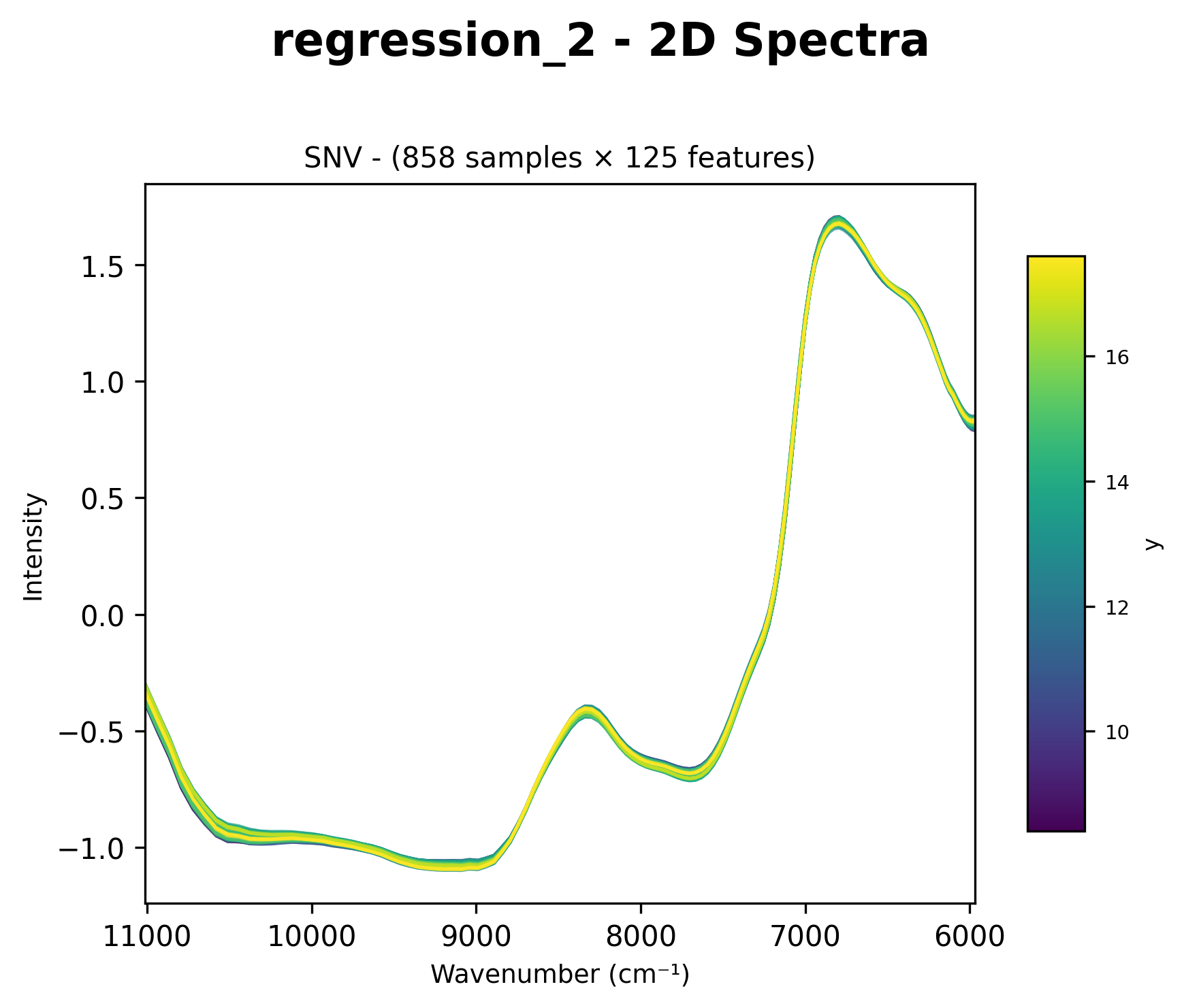
2D Spectra (chart_2d)

Displays all spectra as overlaid lines with color gradient based on y values.

pipeline = [
    "chart_2d",              # Raw spectra
    StandardNormalVariate(),
    "chart_2d",              # After preprocessing
    ShuffleSplit(n_splits=3),
    PLSRegression(n_components=10),
]

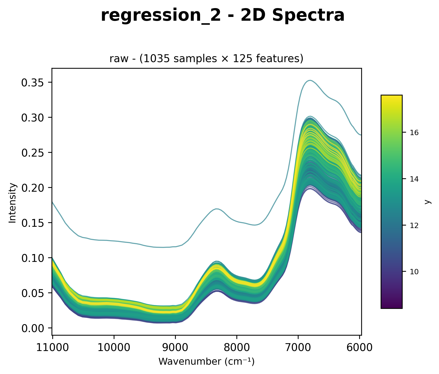
Raw spectral data with color gradient based on target values (wavenumber cm⁻¹ on x-axis).

After Multiple Preprocessing Steps

Place chart_2d after a preprocessing chain to visualize the transformed spectra:

pipeline = [
    StandardNormalVariate(),
    SavitzkyGolay(window_length=11, polyorder=2),
    FirstDerivative(),
    "chart_2d",              # Chart after all preprocessing
    ShuffleSplit(n_splits=3),
    PLSRegression(n_components=10),
]

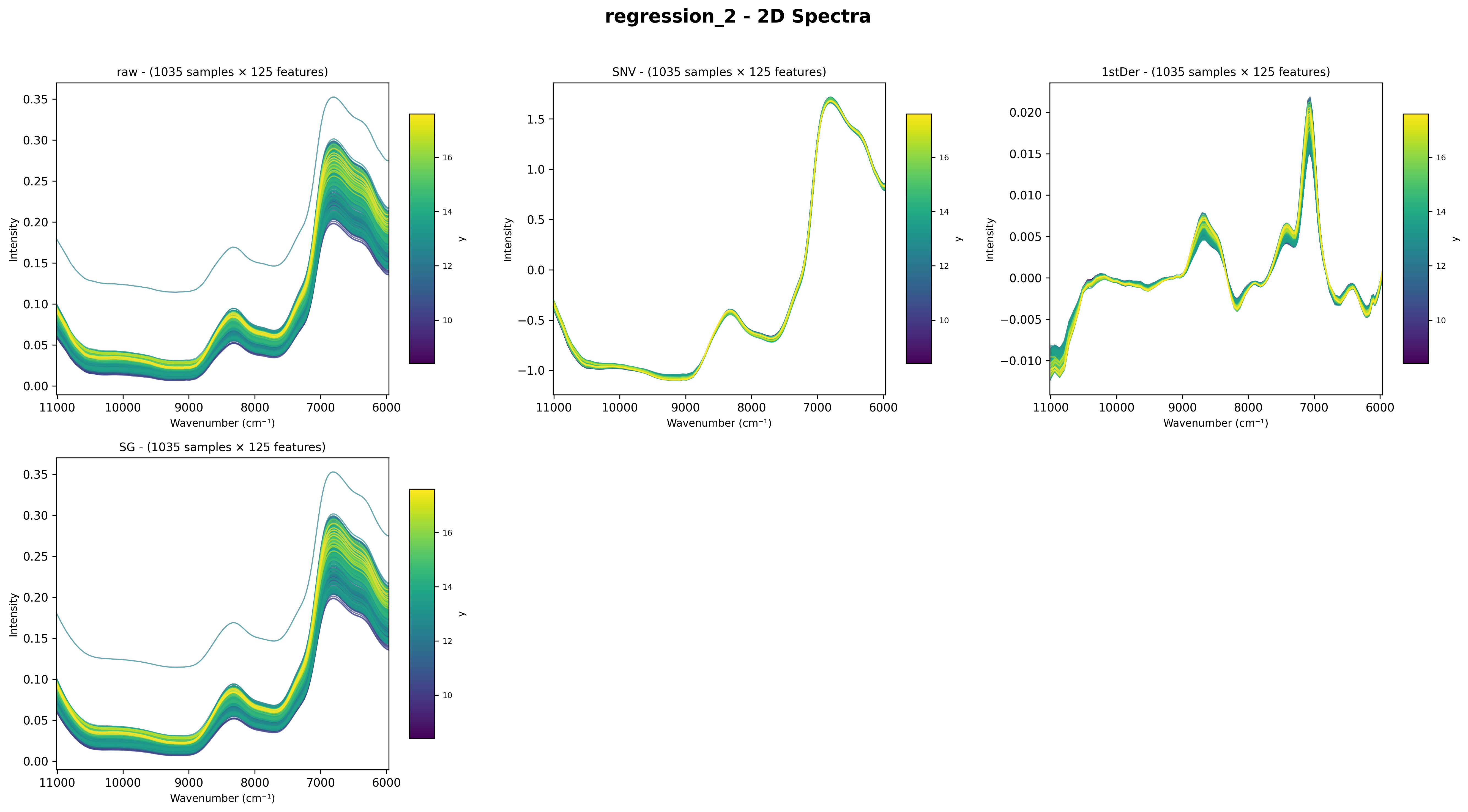
Spectra after SNV + Savitzky-Golay + First Derivative preprocessing.

3D Spectra (chart_3d)

Adds target value as Y-axis for 3D visualization.

pipeline = [
    "chart_3d",              # 3D view with target gradient
    StandardNormalVariate(),
    "chart_3d",
    ShuffleSplit(n_splits=3),
    PLSRegression(n_components=10),
]

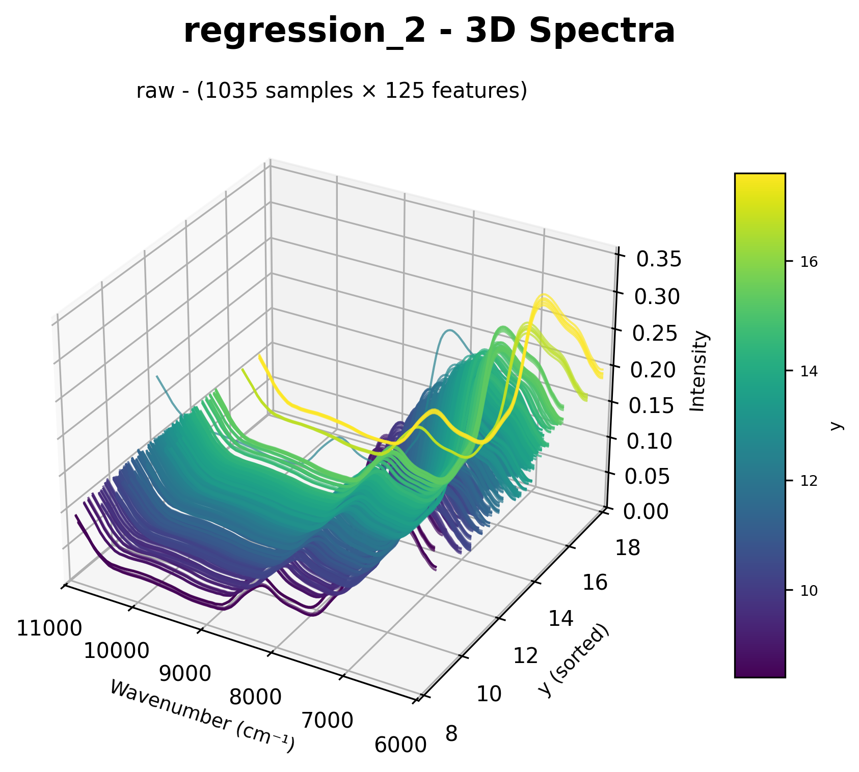
3D spectral visualization with target values as the Y-axis.

Options (Dict Syntax)

{"chart_2d": {
    "include_excluded": True,    # Include excluded samples
    "highlight_excluded": True,  # Highlight excluded with red dashed lines
}}

---

Spectral Distribution Charts

Show statistical envelopes comparing train vs test distributions.

Keywords

• spectral_distribution

• spectra_dist

• spectra_envelope

Usage

pipeline = [
    "spectral_distribution",     # Before preprocessing
    StandardNormalVariate(),
    "spectral_distribution",     # After preprocessing
    ShuffleSplit(n_splits=5),
    PLSRegression(n_components=10),
]

Output:

Shows envelope with:

• Min-max range (light fill)

• IQR range (25th-75th percentile, darker fill)

• Mean line

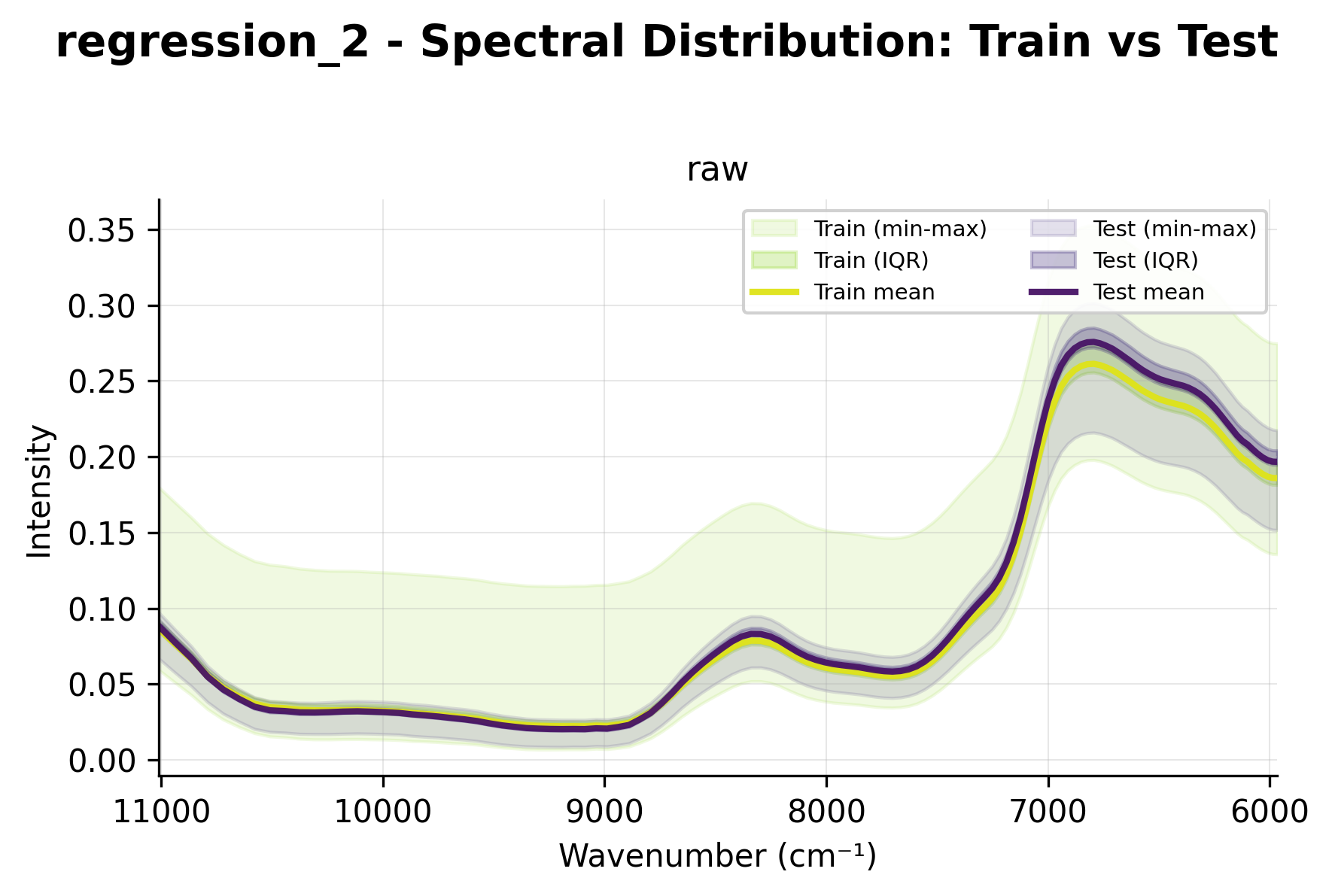
Spectral distribution showing statistical envelopes with wavenumbers on x-axis.

When CV folds exist (> 1), displays a grid with one plot per fold.

---

Fold Charts

Visualize cross-validation fold distributions with color-coded samples.

Keywords

Keyword	Description
fold_chart / chart_fold	Color by y values
fold_<column>	Color by metadata column (e.g., fold_breed)

Usage

pipeline = [
    ShuffleSplit(n_splits=5, test_size=0.2),
    "fold_chart",                # Visualize fold distribution
    PLSRegression(n_components=10),
]

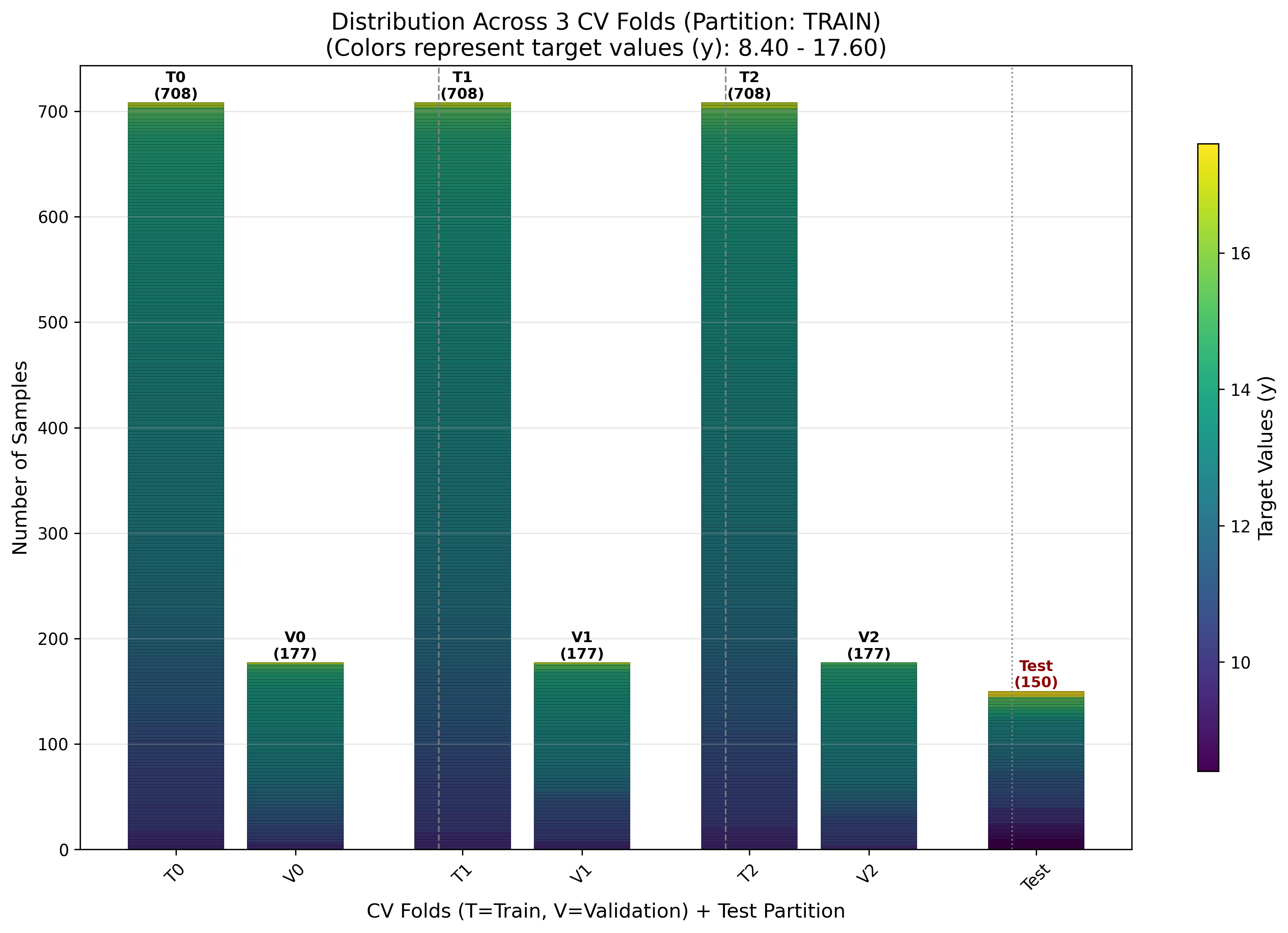
Cross-validation fold distribution with train (T) and validation (V) sets.

• T: Train set for fold

• V: Validation set for fold

• Colors: Gradient based on y values (continuous) or discrete colors (classification)

Color by Metadata Column

pipeline = [
    ShuffleSplit(n_splits=5),
    "fold_breed",                # Color by 'breed' metadata column
    PLSRegression(n_components=10),
]

---

Target (Y) Charts

Visualize y-value distributions as histograms.

Keywords

• y_chart

• chart_y

Usage

pipeline = [
    "y_chart",                   # Before splitting
    ShuffleSplit(n_splits=3, test_size=0.2),
    "y_chart",                   # After splitting (train vs test)
    PLSRegression(n_components=10),
]

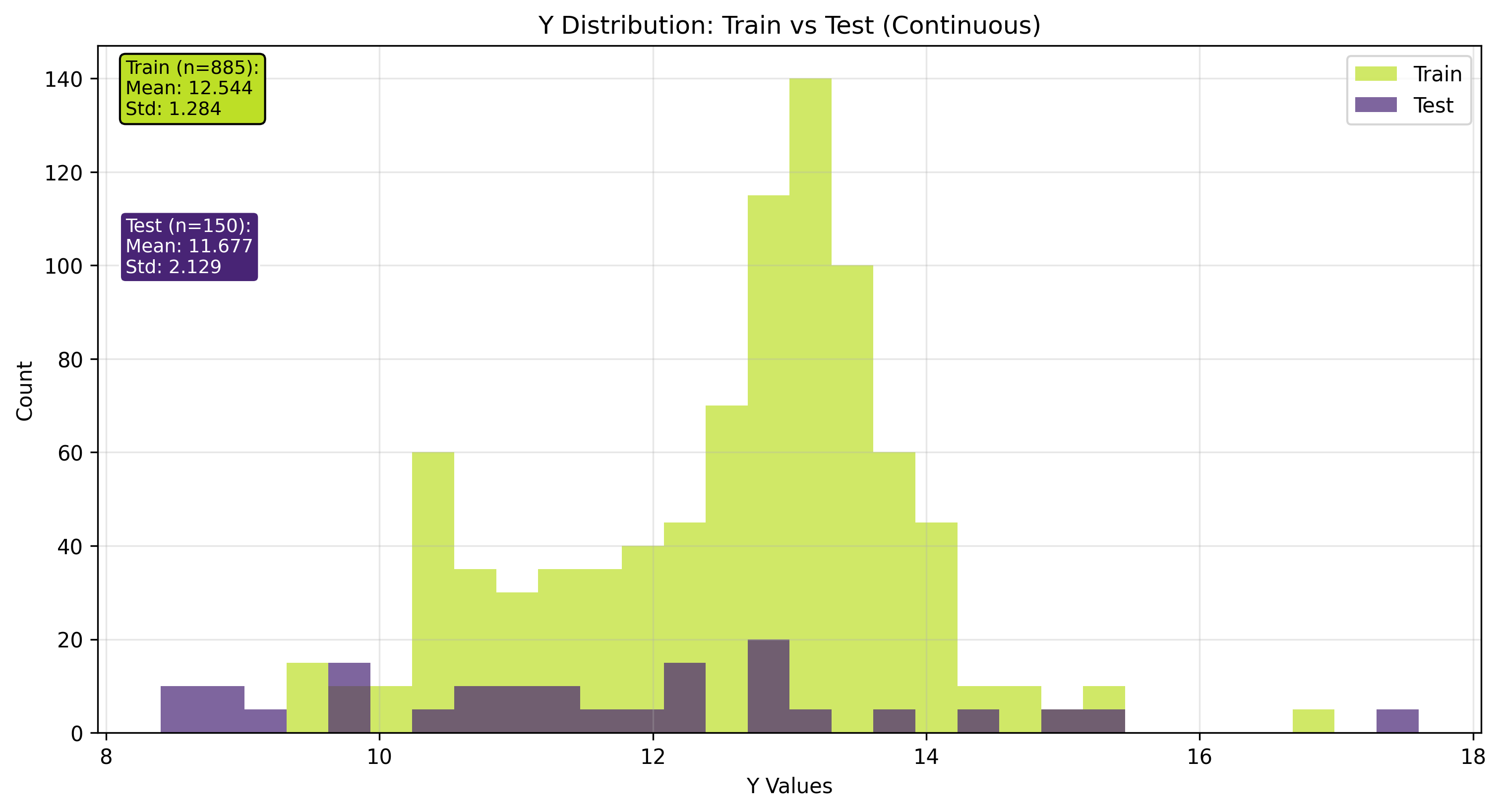
Target value (y) distribution histogram.

Options

{"y_chart": {
    "include_excluded": True,     # Include excluded samples
    "highlight_excluded": True,   # Show excluded as separate histogram
    "layout": "stacked",          # 'standard', 'stacked', or 'staggered'
}}

Layout	Description
standard	Overlapping histograms (default)
stacked	Bars stacked on top of each other
staggered	Side-by-side bars

CV Fold Mode

When multiple CV folds exist, displays a grid with one histogram per fold showing train vs validation distribution.

---

Augmentation Charts

Visualize the effects of sample augmentation.

Keywords

Keyword	Description
augment_chart / augmentation_chart	Overlay of original vs augmented
augment_details_chart / augmentation_details_chart	Grid showing each augmentation type

Usage

from nirs4all.operators.augmentation import GaussianNoise, SpectrumShift

pipeline = [
    {"sample_augmentation": [GaussianNoise(sigma=0.01), SpectrumShift(max_shift=5)]},
    "augment_chart",             # Overlay view
    "augment_details_chart",     # Detailed grid view
    ShuffleSplit(n_splits=3),
    PLSRegression(n_components=10),
]

Overlay Chart (augment_chart)

Shows original spectra with augmented versions overlaid:

• Original samples in solid lines

• Augmented samples in dashed lines with different colors

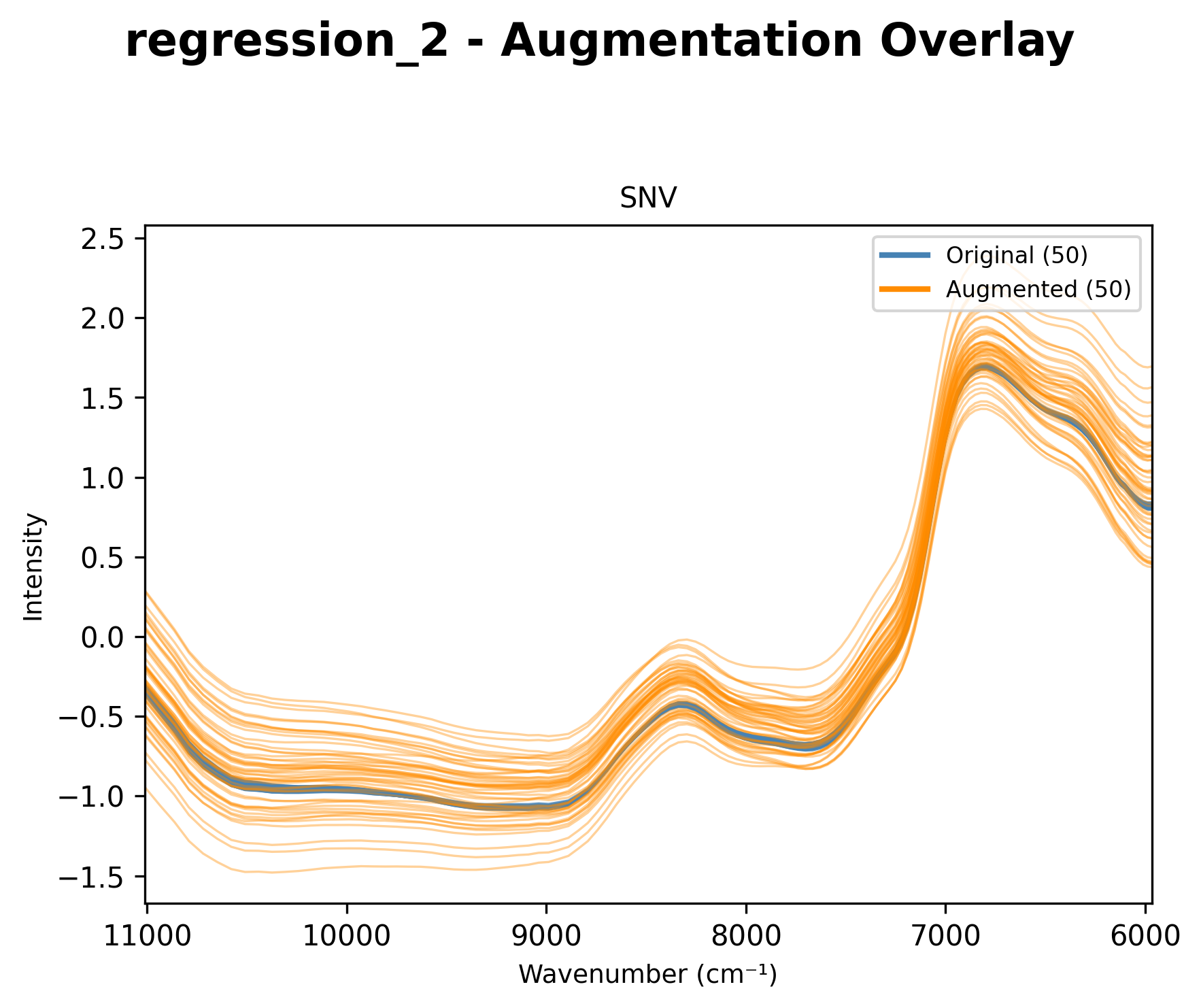
Overlay of original and augmented spectra.

Details Chart (augment_details_chart)

Shows a grid with one subplot per augmentation type:

• First panel: Raw (original) spectra

• Subsequent panels: Each augmentation technique separately

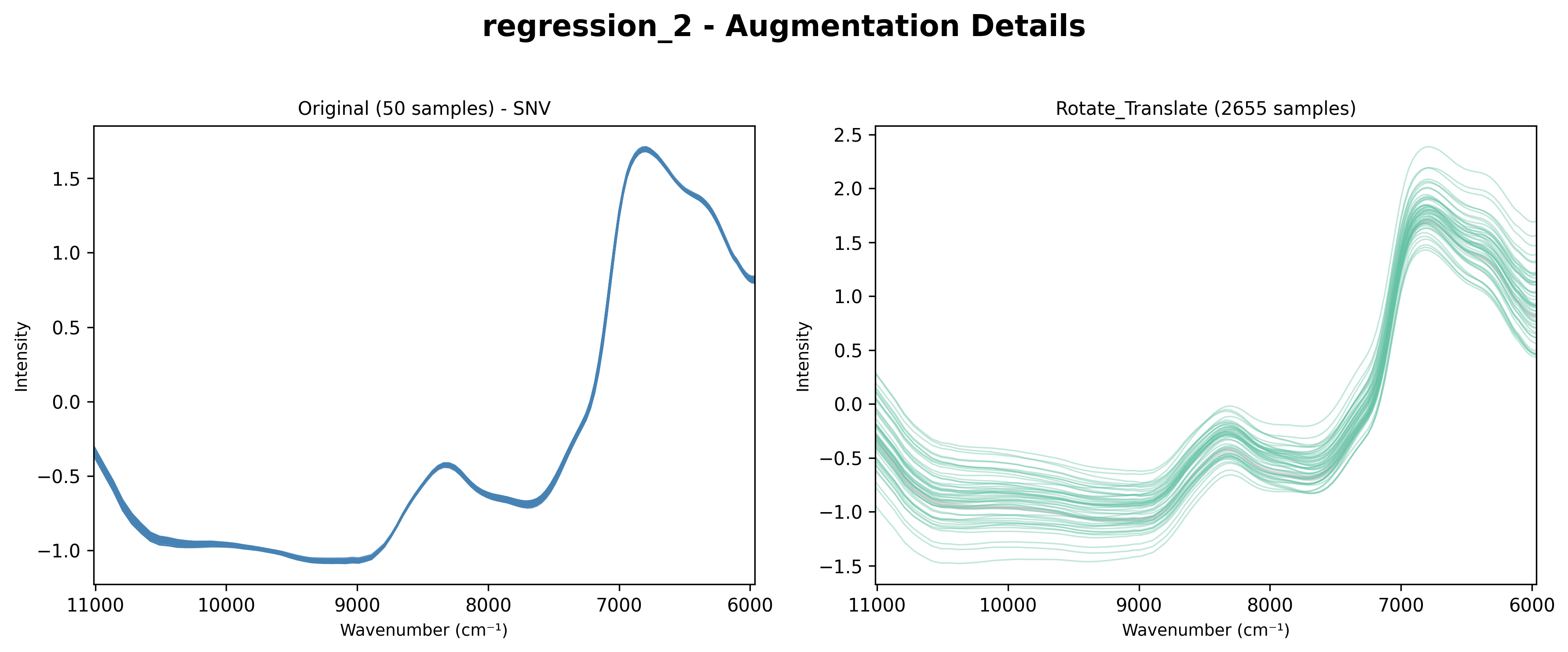
Grid showing each augmentation type separately.

Multiple Augmentation Methods

When using multiple augmentation transformers, the details chart shows each method:

from nirs4all.operators.augmentation import GaussianAdditiveNoise, WavelengthShift

pipeline = [
    {"sample_augmentation": {
        "transformers": [
            GaussianAdditiveNoise(sigma=0.003),
            WavelengthShift(shift_range=(-2, 2)),
        ],
        "count": 2,
    }},
    "augment_chart",
    "augment_details_chart",
    ShuffleSplit(n_splits=3),
    PLSRegression(n_components=10),
]

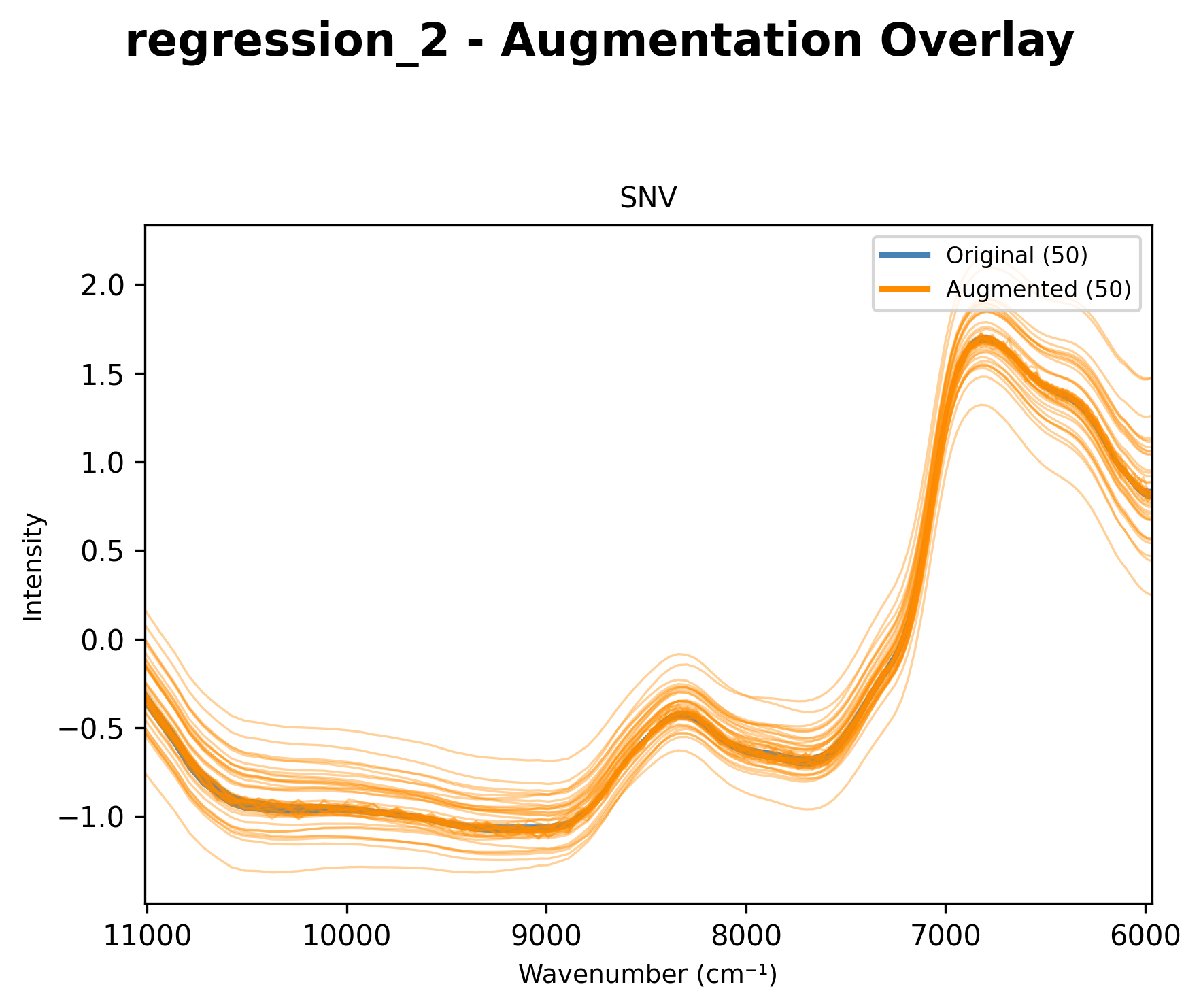
Overlay of original spectra with multiple augmentation methods applied.

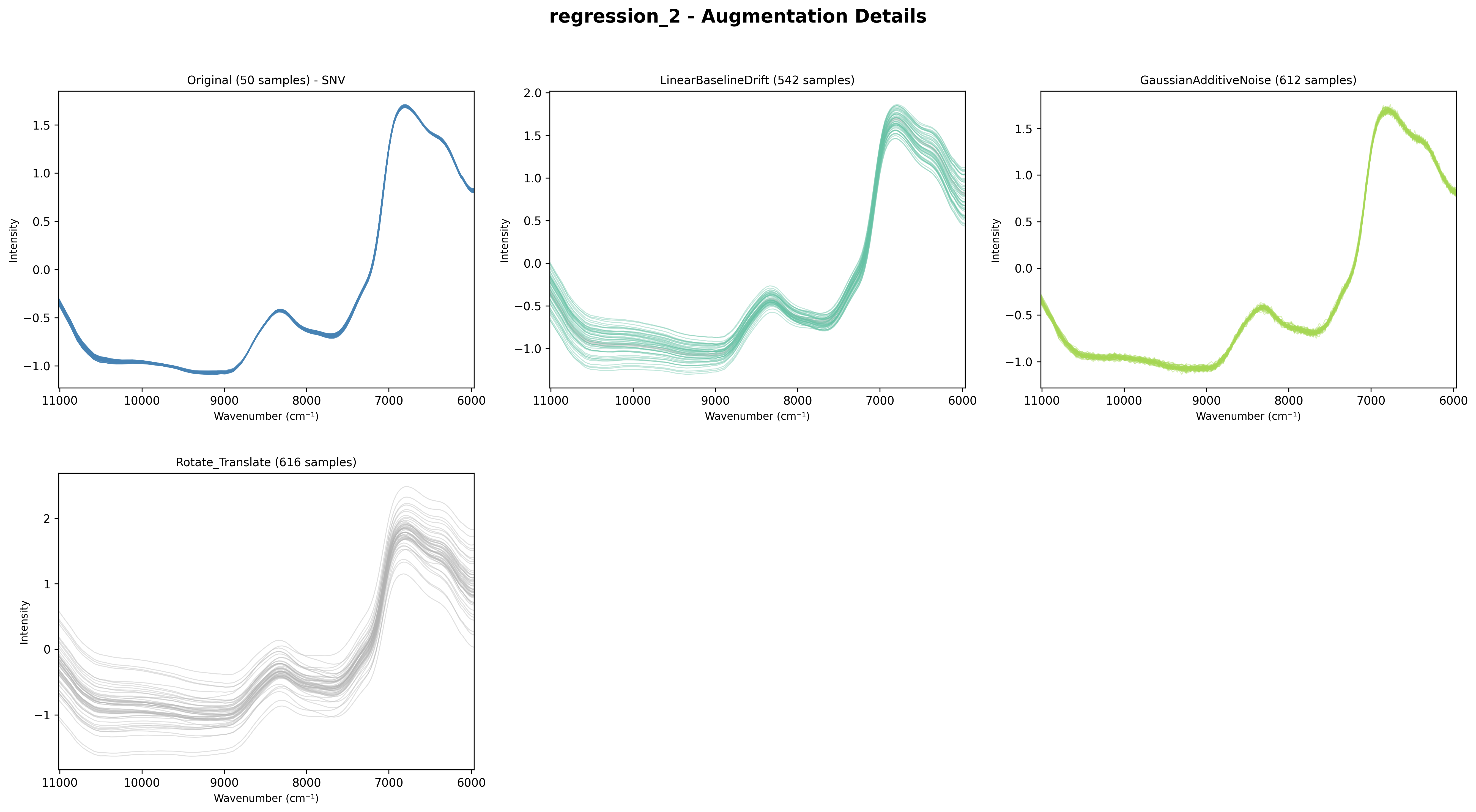
Grid showing each augmentation method (GaussianNoise and WavelengthShift) separately.

---

Exclusion Charts

Visualize included vs excluded samples using PCA projection.

Keywords

• exclusion_chart

• chart_exclusion

Usage

from nirs4all.operators.transforms import OutlierExclusion

pipeline = [
    StandardNormalVariate(),
    "chart_2d",                  # Before exclusion
    {"sample_filter": {
        "filters": [XOutlierFilter(method='isolation_forest', contamination=0.1)],
    }},
    "exclusion_chart",           # Visualize exclusions
    "chart_2d",                  # After exclusion
    ShuffleSplit(n_splits=3),
    PLSRegression(n_components=10),
]

The exclusion chart uses PCA projection to show included vs excluded samples:

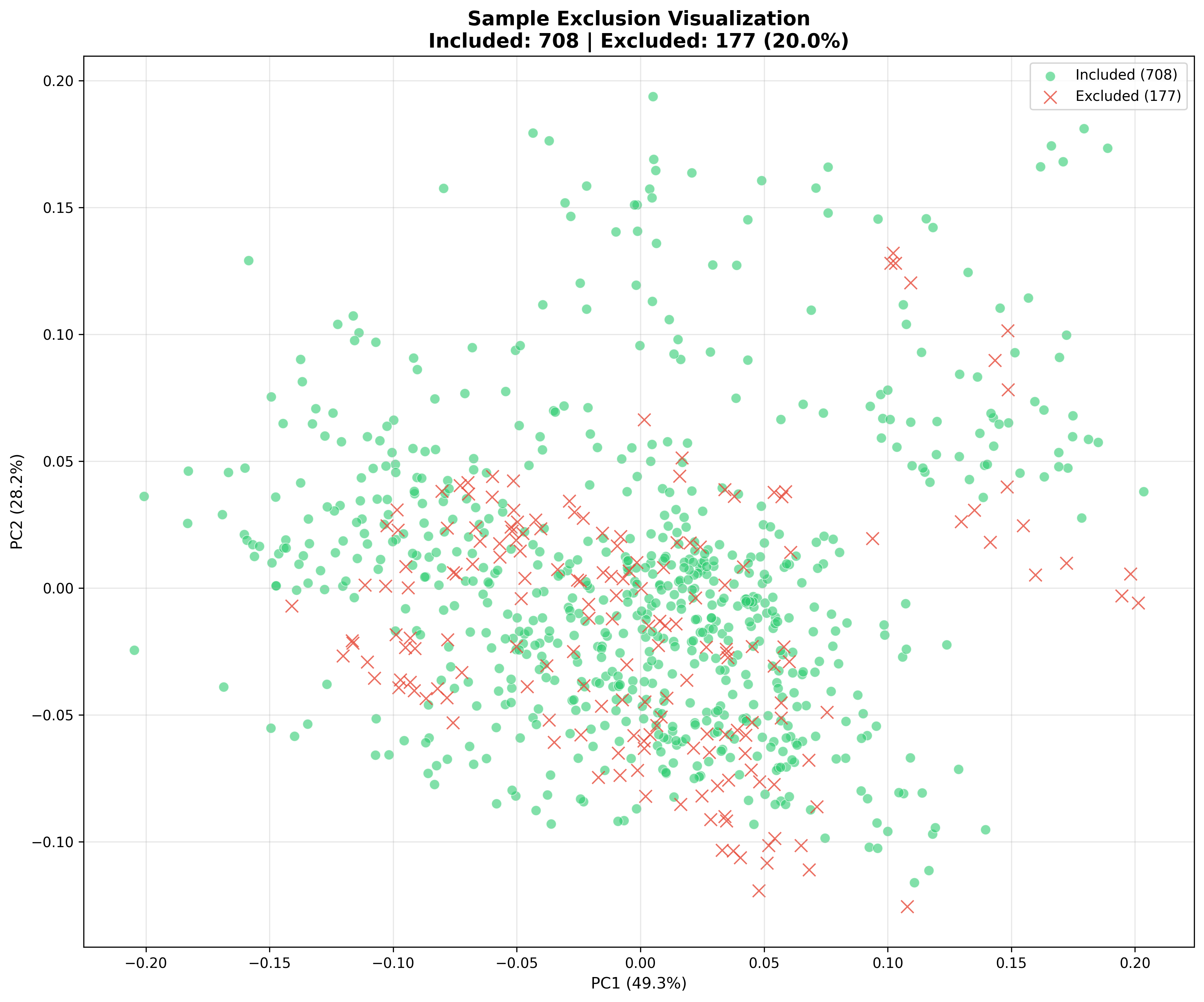
PCA projection showing included (green) vs excluded (red) samples.

Use chart_2d alongside exclusion to see the spectral view of the filtered data:

Spectral view after sample exclusion (outliers removed).

Options

{"exclusion_chart": {
    "color_by": "status",    # 'status', 'y', or 'reason'
    "n_components": 2,       # 2 or 3 for PCA dimensions
    "show_legend": True,
}}

Option	Values	Description
color_by	'status'	Color by included/excluded (default)
	'y'	Color by target value
	'reason'	Color by exclusion reason
n_components	2, 3	PCA dimensions for visualization

---

Controlling Chart Display

Interactive Display

result = nirs4all.run(
    pipeline=pipeline,
    dataset="data/",
    plots_visible=True  # Display plots interactively
)

Save as Artifacts

Charts are automatically saved when using artifacts:

runner = PipelineRunner(
    save_artifacts=True,
    workspace_path="workspace/"
)
predictions, _ = runner.run(pipeline, dataset)
# Charts saved in: workspace/runs/<run_id>/artifacts/

Headless Mode

For automated pipelines without display:

result = nirs4all.run(
    pipeline=pipeline,
    dataset="data/",
    plots_visible=False  # Save only, don't display
)

---

Complete Example

import nirs4all
from sklearn.cross_decomposition import PLSRegression
from sklearn.model_selection import ShuffleSplit
from nirs4all.operators.transforms import StandardNormalVariate, FirstDerivative
from nirs4all.operators.filters import XOutlierFilter
from nirs4all.operators.transforms import GaussianAdditiveNoise

pipeline = [
    # Visualize raw data
    "chart_2d",
    "y_chart",
    "spectral_distribution",

    # Preprocessing
    StandardNormalVariate(),
    FirstDerivative(),
    "chart_2d",                  # After preprocessing

    # Outlier removal
    {"sample_filter": {
        "filters": [XOutlierFilter(method='isolation_forest', contamination=0.05)],
    }},
    "exclusion_chart",

    # Augmentation
    {"sample_augmentation": {
        "transformers": [GaussianAdditiveNoise(sigma=0.01)],
        "count": 2,
    }},
    "augment_chart",

    # Cross-validation
    ShuffleSplit(n_splits=5, test_size=0.2, random_state=42),
    "fold_chart",                # Fold distribution
    "y_chart",                   # Y distribution per fold

    # Model
    {"model": PLSRegression(n_components=10)},
]

result = nirs4all.run(
    pipeline=pipeline,
    dataset="sample_data/regression",
    plots_visible=True,
    save_artifacts=True,
)

---

Best Practices

1. Place strategically: Add charts before and after key transformations

2. Use sparingly in production: Charts add execution time

3. Check distributions: Use spectral_distribution and y_chart to verify train/test similarity

4. Monitor folds: Use fold_chart to ensure balanced CV splits

5. Track exclusions: Always visualize after outlier removal with exclusion_chart

6. Save artifacts: Enable save_artifacts=True for reproducibility

---

See Also

• Analyzer Charts Reference - Post-prediction visualization with PredictionAnalyzer

• SHAP Analysis for NIRS Models - SHAP-based model explanation

• Pipeline Diagram - Pipeline structure visualization

• Preprocessing Overview - Preprocessing techniques